Introduction

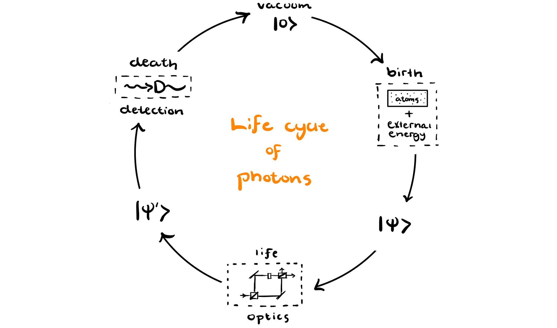
From the vacuum, different quantum states of light are born. We will become familiar with the various states of light as we study the field of quantum optics. We will learn how different states are born, how they evolve, and inevitably how they die (upon detection). In fact, the analysis of a typical quantum optics experiment can just be thought of as the study of the life cycle of photons.

Life cycle of photons.

Quantum optics: the life cycle of photons (figure inspired by Haixing Miao's course notes).

We want to be able to describe this life cycle with more than just words. Like all good stories, that of the photon's birth, life, and death is more exciting in pictures. So, to aid our understanding, we will introduce a mathematical formalism that comes with a clean visualization of quantum states of light. In addition to being pretty to look at, the pictures will also aid in our understanding. The math underlying the pictures will also be useful in computing physically relevant quantities. So, without further adieu, we begin our study of Wigner functions and optical phase space.

Wigner functions and optical phase space

First introduced in 1932 by the great Hungarian physicist Eugene Wigner, the Wigner function is a mathematical object known as a quasi-probability distribution. Why quasi? Well, a probability distribution has to satisfy certain axioms (due to Andrey Kolmogorov). A quasi-probability distribution allows these axioms to be relaxed. As we will see, Wigner functions can be negative, a feature certainly not allowed of a classical probabiltiy distribution. Nonetheless, I maintain that the Wigner function is a useful mathematical tool. Okay, enough talk, let's do some math.

The Wigner function

The Wigner function is a map from the space of quantum states to optical phase space. If you have studied classical mechanics at the advanced undergraduate or graduate level, you have probably used phase space to study the solutions to the Euler-Lagrange equations of motion. For example, the solution of the simple harmonic oscillator can be represented in phases space as (insert figure)

where here \(x\) and \(p\) are the position and momentum variables, respectively. Optical phase space is just like normal phase space except position and momentum variables are replaced by the amplitude and phase quadrature operators defined as

\[X=\frac{a+a^{\dagger}}{\sqrt{2}} \quad \text{and} \quad Y=\frac{a-a^{\dagger}}{i\sqrt{2}}.\]

The Wigner function is defined as

\[W(X,Y)= \frac{1}{\pi} \int_{-\infty}^{\infty} \langle X+X'| \psi \rangle \langle \psi | X-X' \rangle e^{-2i X' Y} dX'.\]

The first time I saw this I was thoroughly confused. It looked ever-so-slightly like a Fourier transform but overall I just was not sure what to make of it. When meeting a very general mathematical object for the first time, it is very often a good idea to plug in specific inputs and see if you can make some sense of things. The input to this function is a quantum state \(|\psi \rangle\), so why don't we start by considering the simplest quantum state?

Visualizing quantum states of light: optical phase space

The vacuum state \(|0\rangle \), is perhaps the simplest quantum state to study. It represents the absence of excitations and to compute the vacuum Wigner function, we simply need to know the overlaps \(\langle X+X'| \psi \rangle\) and \(\langle \psi | X-X' \rangle \). Because the quantized electromagnetic field is mathematically equivalent to a quantum harmonic oscillator, the wavefunctions we desire are simply the ground state wave functions of a harmonic oscillator:

\[\langle X+X'| \psi \rangle = \left(\frac{1}{\pi}\right)^{1/4} e^{-\frac{(X+X')^2}{2}},\]

and

\[\langle X-X' |\psi \rangle = \left(\frac{1}{\pi} \right)^{1/4} e^{-\frac{(X-X')^2}{2}}.\]

If these are unfamiliar, I recommend reading Chapter 2 Section 4 of Introduction to Quantum Mechanics by David J. Griffiths or taking my word for it. Note, in quantum optics, wuantities of interest are usually defined so as to simplify mathematical results and free them from pesky physical constants. So, if you are comparing to Griffiths, there may be some \(\hbar\)'s and \(\omega\)'s missing. In our notation, though, the ground state Wigner function becomes

\[\begin{aligned} W_0 (X,Y) &= \frac{1}{\pi} \int_{-\infty}^{\infty} \left[\left(\frac{1}{\pi}\right)^{1/4} e^{-\frac{(X+X')^2}{2}} \right] \left[ \left(\frac{1}{\pi} \right)^{1/4} e^{-\frac{(X-X')^2}{2}} \right] e^{-2i X' Y} dX',\\ W_0 (X,Y) &=\left(\frac{1}{\pi} \right)^{3/2} \int_{-\infty}^{\infty} e^{-\frac{(X+X')^2}{2}} e^{-\frac{(X-X')^2}{2}} e^{-2i X' Y} dX',\\ W_0 (X,Y) &=\frac{1}{\pi} e^{-(X^2 +Y^2)} \end{aligned}\]

Wigner function and optical phase space representation.

What good is a quasi-probability distribution?

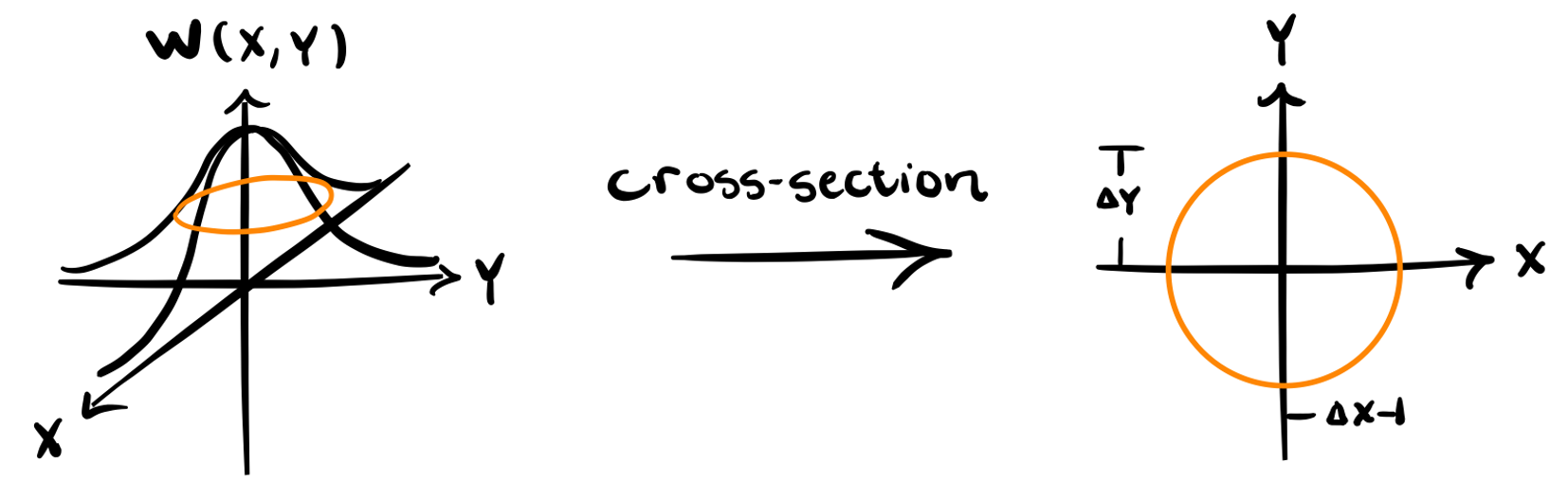
First and foremost, the cross-section of the Wigner functions provide a great visual tool to understanding quantum states of light. This fact is best appreciated after we meet several quantum states of light. However, in addition to the instructive nature of phase space diagrams, the Wigner functions themselves can be use to calculate quantities of interest with ease. Recall, that the expectation value of a classical continuous random variable is simply

\[\begin{aligned} \langle x \rangle &= \int p(x) x dx, \end{aligned}\]

where the integral is taken over the relevant space. As we will see, the Wigner function allows us to compute quantities in nearly the same manner. For example, let's say we wish to compute the correlation between the amplitude and phase quadratures. Why would we be interested in this quantity? Well, in quantum optics, if we can produce correlated observables, we can often make use of these correlations to obtain higher precision in measurements. So, whenever we meet a new quantum state, the natural question is often "are the ampitude and phase quadratures correlated?" And while there are many ways to compute these quantites, in order to see the power of the Wigner function, we will use it to compute the covariance of the amplitude and phase quadratures for a vacuum state.

Covariance of amplitude and phase quadratures of a vacuum state

First, recall that the correlation between two classical random variables, say \(x\) and \(y\), is defined as

\[\begin{aligned} \text{corr(x,y)}&= \frac{\langle xy \rangle -\langle x \rangle \langle y \rangle}{\sigma_x \sigma_y}, \end{aligned}\]

where \(\langle x \rangle\), \(\sigma_x\) denote the average value and the the standard deviation of the random variable \(x\), respectively. Correlation can be thought of as a normalized covariance. Sometimes it is more convenient to work with covariance and not worry about normalization. As a reminder, the covariance of random variables \(x\) and \(y\) is just given as

\[\begin{aligned} \text{cov(x,y)}&= \langle xy \rangle -\langle x \rangle \langle y \rangle. \end{aligned}\]

Both, however, measure dependence of one variable on another and are used widely. Now, in quantum mechanics, observables do not always commute. That is, \(XY\) need not always equal \(YX\). To account for this issue when making a classical formula quantum, one must symmetrize products of operators. In our case, the symmetrized covariance of two quantum observables \(X,Y\) is given as

\[\begin{aligned} \text{cov(x,y)}&= \langle \frac{1}{2}(XY+YX) \rangle -\langle X \rangle \langle Y \rangle. \end{aligned}\]

We see that if \(X\) and \(Y\) do commute then \(\frac{1}{2}(XY+YX)=XY\), but this need not be the case in general. Now, the beauty of the Wigner function is that, just as in classical probability theory, we can compute the expectation values by integrating against the, in the quantum case, quasi probability distribution function. Let's do so for each term in the covariance formula

\[\begin{aligned} \frac{1}{2} \langle XY \rangle &= \frac{1}{2} \int_{-\infty}^{\infty}\int_{-\infty}^{\infty} W(X,Y) XY dX dY, \\ \frac{1}{2} \langle YX \rangle &= \frac{1}{2} \int_{-\infty}^{\infty}\int_{-\infty}^{\infty} W(X,Y) XY dX dY, \\ \langle X\rangle &= \int_{-\infty}^{\infty}\int_{-\infty}^{\infty} W(X,Y) X dX dY, \\ \langle Y \rangle &=\int_{-\infty}^{\infty}\int_{-\infty}^{\infty} W(X,Y) Y dX dY. \\ \end{aligned}\]

Then, substituting in the vacuum state Wigner function, we see

\[\begin{aligned} \frac{1}{2} \langle XY \rangle &= \frac{1}{2} \int_{-\infty}^{\infty}\int_{-\infty}^{\infty} \left(\frac{1}{\pi} e^{-(X^2 +Y^2)} \right) XY dX dY=0, \\ \frac{1}{2} \langle YX \rangle &= \frac{1}{2} \int_{-\infty}^{\infty}\int_{-\infty}^{\infty} \left(\frac{1}{\pi} e^{-(X^2 +Y^2)} \right) XY dX dY=0, \\ \langle X\rangle &= \int_{-\infty}^{\infty}\int_{-\infty}^{\infty} \left(\frac{1}{\pi} e^{-(X^2 +Y^2)} \right) X dX dY=0, \\ \langle Y \rangle &=\int_{-\infty}^{\infty}\int_{-\infty}^{\infty}\left(\frac{1}{\pi} e^{-(X^2 +Y^2)} \right) Y dX dY=0.\\ \end{aligned}\]

Because, in every case, we are integrating an odd function over a symmetric range around zero the integrals are zero and we conclude that the quadratures of a vacuum state are uncorrelated

\[\text{cov}(X,Y) = \text{corr}(X,Y) = 0.\]

This is an interesting result, as we will come to appreciate when we explore quantum optics experiments. Vacuum states are to most quantum optics experiments what guys with acoustic guitars are to most parties: an unwanted feature that everyone learns to deal with. Vacuum fluctuations are inevitable in any experiment and actually set what is called the standard quantum limit to an experiment. To surpass this limit, we have to engineer states of light that do have correlations between their quadratures.

Using the Wigner function is nice because it so directly parallels classical methods. However, I very briefly want to show another standard method for calculating these quantites.

Covariance matrices

Linear algebra is perhaps the most important field of mathematics someone interested in quantum optics, quantum information, etc could study. As usual, its application to the problem at hand leads to an elegant result. The covariance matrix elements are defined as (Eq. 15 in this beautiful review):

\[\begin{aligned} V_{ij}:= \frac{1}{2} \langle \{\Delta X_i, \Delta X_j\} \rangle, \end{aligned}\]

where \(\Delta X_i := X_i - \langle X_i \rangle\) and \(\{A,B\}:=AB+BA\) is the anti-commutator of the operators \(A\) and \(B\). Remember that for the vacuum state both the amplitude and phase quadratures average to zero. The beauty of phase space pictures introduced above is we just need to remember that the vacuum state is a circle centered on the origin and this reminds us that the expectation values are zero. Thus, for amplitude and phase quadratures \(X\) and \(Y\), the full covariance matrix becomes

\[\begin{aligned} V_0 &= \frac{1}{2}\begin{bmatrix} \langle 0 |\{\Delta X,\Delta X\} |0\rangle & \langle 0 |\{\Delta X,\Delta Y\}|0\rangle \\ \langle 0 |\{\Delta Y,\Delta X\}|0\rangle & \langle 0 |\{\Delta Y,\Delta Y\}|0\rangle \end{bmatrix},\\ &= \begin{bmatrix} \langle 0 | X^2 |0\rangle & \langle 0 |XY+YX|0\rangle \\ \langle 0 |YX+XY|0\rangle & \langle 0 |Y^2|0\rangle \end{bmatrix}. \end{aligned}\]

Then, we just need to expand these operators and use the rules for creation and annihilation operators acting on number states to simplify this fully. I will do one and leave the others as an exercise. We have

\[\begin{aligned} \langle 0 | X^2 |0\rangle &= \langle 0 | \left(\frac{a+a^{\dagger}}{\sqrt{2}}\right)\left(\frac{a+a^{\dagger}}{\sqrt{2}}\right) |0\rangle, \\ &= \frac{1}{2}\langle 0 | \left(aa+aa^{\dagger}+a^{\dagger}a +a^{\dagger}a^{\dagger}\right) |0\rangle,\\ &= \frac{1}{2}\left(\langle 0 |aa|0\rangle+\langle 0|aa^{\dagger}|0\rangle+\langle 0|a^{\dagger}a|0\rangle +\langle 0|a^{\dagger}a^{\dagger}|0\rangle \right),\\ &= \frac{1}{2}\left(0+1+0+0\right),\\ \langle 0 | X^2 |0\rangle &= \frac{1}{2}. \end{aligned}\]

As you will find, the final covariance matrix for the vacuum state is

\[\begin{aligned} V_0 &= \begin{bmatrix} \frac{1}{2} & 0\\ 0 & \frac{1}{2} \end{bmatrix}. \end{aligned}\]

A diagonal covariance matrix is characteristic of a state without correlations between quadratures. In a future post, we will see that this indicates there is no entanglement in the system. Although there is not entanglment, the vacuum state is still a minimum uncertainty state in that it saturates the Heisenberg uncertainty relation (\(\Delta X \Delta Y \geq \frac{1}{2}\), in our normalization). We can see this by simply taking the determinant of our covariance matrix:

\[\begin{aligned} \text{det}[V_0] &=\left|\begin{bmatrix} \frac{1}{2} & 0\\ 0 & \frac{1}{2} \end{bmatrix}\right|,\\ &= \frac{1}{4}. \end{aligned}\]

The diagonal terms of the covariance matrix are simply variances of the quadratures, so from the above we can conclude that \(V(X)V(Y)=1/4\) and thus taking the square root of both sides yields

\[\begin{aligned} \Delta X \Delta Y = \frac{1}{2}, \end{aligned}\]

which saturates the Heisenberg uncertainty principle. One may think, then, that this is the best we can do. Just make sure any unwanted field is in a vacuum state and that will give minimum uncertainty. Operating under this assumption would put you at the standard quantum limit mentioned above. However, one of the most amazing features of quantum optics is that we can actually surpass the standard quantum limit by squeezing light. Doing so keeps one in a minimum uncertainty state but moves some uncertainty out of one quadrature and into the other. Thus, Heisenberg is happy but we get increased sensitivity in one quadrature. The importance of this method can't be overstated and we will explore it in depth in future posts.

Summary

Key take-aways

If nothing else, I hope you take away the following points:

Wigner functions are a quasi-probability distribution because they relax some of the axioms of probability,
They are useful objects because they can be used like classical probability distributions to compute expectation values,
Optical phase space diagrams are used ubiquitously throughout quantum optics literature and are generated by taking the cross section of a Wigner function,
The vacuum state is a minimum uncertainty state with uncorrelated amplitude and phase quadratures.

Suggested resources

This post assumed some knowledge of quantum harmonic oscillators. If you are unfamiliar with this topic, I recommend Griffiths textbook. If you want to learn more about the quantized electromagnetic field, I would try Gerry and Knight's quantum optics textbook first, though there are many good options. For general info on phase space, covariance, correlation, etc. I recommend starting with Wikipedia and going from there!