Background

In 1967, Carl W. Helstrom (1925-2013) published a paper entitled Minimum mean-squared error of estimates in quantum statistics. The more I have studied quantum metrology, the more I have come to appreciate this paper's significance in the field. Because of its brevity and importance, I thought it would be perfect for the first paper walk-through on this site. In all paper walk-throughs I am essentially just sharing my understanding of a published paper. Due to many factors, published papers can be very difficult for young researchers to understand. I want to rectify this for a tiny subset of papers I enjoy and think I understand well enough. When open-source versions of paper's exist, I will link to them. Sadly, this seminal work long predated the arXiv, so I will re-derive the key results and hope you can find a copy somewhere. Let's get started with some preliminaries!

Useful Facts

We start by stating a few facts that are crucial to understanding Helstrom's brief paper. For the sake of brevity, I will link either to separate posts on relevant topics or external sites for more information and/or proofs.

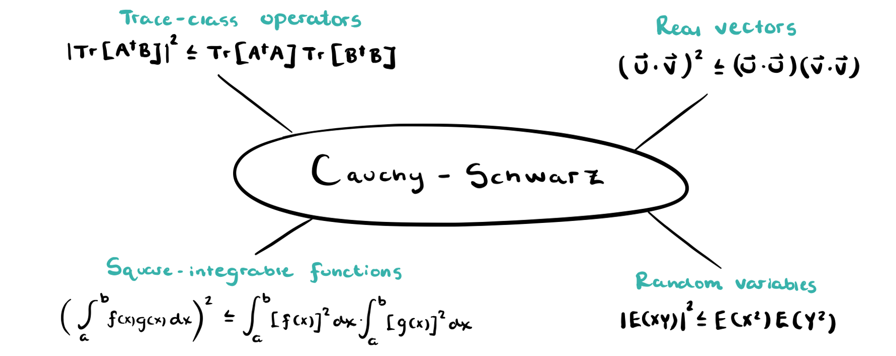
Cauchy-Schwarz Inequality

A ubiquitous tool in linear algebra is called the Cauchy-Schwarz inequality. As shown in the figure below, the inequality can take many different forms.

We now state the general result (see this great site for various proofs).

Let $V$ be a vector space and let $\langle \cdot,\cdot \rangle: V \times V \rightarrow \mathbb{F}$ be an inner product. Here $\mathbb{F}$ denotes a general number field. In our case, though, we will have $\mathbb{F}=\mathbb{C}$. Then for $\mathbf{v},\mathbf{u} \in V$,

$$|\langle \mathbf{v},\mathbf{u} \rangle|^2 \leq \langle \mathbf{v},\mathbf{v} \rangle \langle \mathbf{u},\mathbf{u} \rangle, $$

with equality iff one of $\mathbf{u},\mathbf{v}$ is a scalar multiple of the other. This holds for any general inner product; however, we will specifically need it as applied to the Hilbert-Schmidt inner product.

For two operators $A,B$ in a Hilbert space $\mathcal{H}$, the Hilbert-Schmidt inner product is defined as $\langle A,B \rangle_{\text{HS}} = \text{Tr}[A^{\dagger}B]$. So, the Cauchy-Schwarz inequality becomes

$$ |\text{Tr}[A^{\dagger}B]|^2 \leq \text{Tr}[A^{\dagger}A]\text{Tr}[B^{\dagger}B].$$

Properties of Trace

The Trace of a square matrix is simply the sum of the diagonal elements. The trace is linear. That is, for two trace-class operators $A,B$,

$$ \text{Tr}[A+B]=\text{Tr}[A]+\text{Tr}[B],$$

and

$$\text{Tr}[cA]=c\text{Tr}[A].$$

In general, the trace of an operator is a complex number. So, we have

$$\text{Tr}[A]=z \implies \text{Tr}[A^{\dagger}]=z^*.$$

Finally, the trace is invariant under cyclical permutations. For three trace-class operators $A,B,C \in \mathcal{H}$

$$\text{Tr}[ABC]=\text{Tr}[BCA]=\text{Tr}[CAB].$$

Quantum states and expectation values

The normalization of a quantum state $\rho \in \mathcal{H}$ can be expressed as

\[ \text{Tr}[\rho]=1.\]

The expectation value of an operator $A \in \mathcal{H}$ with respect to a quantum state $\rho$ is

\[\langle A \rangle_{\rho}= \text{Tr}[\rho A].\]

Properties of complex numbers

Let us denote a complex number $z\in \mathbb{C}$ as $z=a+bi$ for $a,b \in \mathbb{R}$. Then, the real part, denoted $\text{Re} [z]$ is given as

\[ a := \text{Re} [z] = \frac{z+z^*}{2}.\]

A final fact we will need is an intuitive one. The real part of a complex number is never larger than the magnitude of the complex number itself. Denoting the magnitude of the complex number as $|z| = \sqrt{a^2 +b^2}$, we have

\[|z|^2 = a^2 + b^2 \geq a^2.\]

This fact seems obvious, but is used in the derivation so we state it for convenience. Now, with these facts in mind, we can derive the quantum Cramer-Rao bound (QCRB) as Helstrom did over 50 years ago.

Deriving the QCRB

Definitions

Let $\rho = \rho(\theta)$ be a quantum state that depends on an unknown parameter we wish to estimate. For example, $\theta$ could represent magnetic field strength or temperature. Then, let $X$ be a Hermitian operator corresponding to some quantum observable. Carrying out this measurement leads to an approximation of $\theta$ which is canonically denoted $\hat{\theta}$. Ideally, this estimator will equal the unknown parameter on average, $E(\hat{\theta}) = \text{Tr}[\rho X]$. This is the situation many modern works on QCRB treat. However, Helstrom allowed for a bias defined simply as the difference between the actual parameter $b(\theta) = E(\hat{\theta}) - \theta$. We can re-express this as

\[\begin{aligned} b(\theta) &= E(\hat{\theta}) - \theta, \\ &= \text{Tr}[\rho X] - \text{Tr}[\rho \theta], \quad & \text{Tr}[\rho]=1 \text{ and linearity of trace} \\ b(\theta)&=\text{Tr}[\rho (X-\theta)], \quad & \text{linearity of trace}. \end{aligned}\]

The quantum Cramer-Rao bound

After these definitions, Helstrom claims that the mean-squared error of an observable $E(\hat{\theta}-\theta)^2= \text{Tr}[\rho(X-\theta)^2]$ must satisfy

\[\boxed{ \text{Tr}[\rho(X-\theta)^2] \geq \frac{(1+b'(\theta))^2}{\text{Tr}[\rho L^2]},}\]

where $b'(\theta)$ is the derivative of the bias with respect to $\theta$ and the operator $L$ is the called the symmetric logarithmic derivative (SLD) and satisfies the operator differential equation

$$\frac{\partial\rho}{\partial \theta}=\frac{1}{2}(\rho L + L \rho).$$

For now, take this equation as a definition that will be used in mathematical manipulations. In a later post, we will understand all components of this inequality in better detail.

Proof of the QCRB

Now, if asked to prove this without the help of Helstom's paper, how might we do it? For starters, we can find an expression for the derivative of the bias in terms of traces. We can write

$$\begin{aligned} \frac{d b(\theta)}{d \theta} &= \frac{d}{d \theta}\left[ \text{Tr}[\rho(X-\theta)]\right] \\ &= \text{Tr}\left[\frac{d}{d \theta} [\rho(X-\theta)]\right] \\ &= \text{Tr} \left[ \frac{d\rho}{d\theta}X\right] -\text{Tr} \left[ \frac{d\rho}{d\theta}\theta\right] + \text{Tr} \left[ \rho \frac{dX}{d\theta}\right] - \text{Tr} \left[ \rho \frac{d\theta}{d\theta}\right], \quad & \text{ product rule and linearity of trace}\\ &= \text{Tr} \left[ \frac{d\rho}{d\theta}X\right] - \theta \frac{d}{d \theta} \left[\text{Tr}[\rho] \right] + 0 - 1, \quad & X \text{ is parameter-independent and Tr}[\rho]=1 \\ \end{aligned}$$

and rearranging we have

\[1+b'(\theta) = \text{Tr}\left[\frac{\partial \rho}{\partial \theta} X \right].\]

Now, the right-hand side of the QCRB has a numerator of $(1+b'(\theta))^2$, so we may be tempted to square this expression and manipulate from there. However, we also need to get the $(X-\theta)^2$ term somehow. Helstrom's clever trick, one that is used frequently throughout mathematics, is to subtract zero in a clever way. In this case, note $\text{Tr}[\rho]=1$ implies $\text{Tr}[\partial \rho /\partial \theta]=0$, which further implies $\text{Tr}[\frac{\partial \rho}{\partial \theta} \theta]=0$. Now, we can write

\[\begin{aligned} 1+b'(\theta) - 0 &= \text{Tr}\left[\frac{\partial \rho}{\partial \theta} X \right] - \text{Tr}\left[\frac{\partial \rho}{\partial \theta} \theta\right],\\ 1+b'(\theta)&= \text{Tr}\left[\frac{\partial \rho}{\partial \theta} (X-\theta)\right]. \end{aligned}\]

Now squaring both sides in hopes of using Cauchy-Schwarz, we have

\[\begin{aligned} (1+b'(\theta))^2&= \left(\text{Tr}\left[\frac{\partial \rho}{\partial \theta} (X-\theta)\right] \right)^2, \\ &= \left(\text{Tr}\left[\left(\frac{1}{2} (\rho L + L\rho)\right) (X-\theta)\right] \right)^2, \quad & \text{ definition of the SLD} \\ &= \left( \frac{1}{2} \left(\text{Tr}\left[\rho L(X-\theta)\right] +\text{Tr}\left[ (X-\theta)L\rho\right] \right)\right)^2,\\ \end{aligned}\]

where in the last line we use both linearity and cyclicity of the trace. Now, noting that all operators involved here are Hermitian we can identify $$A=\rho L (X-\theta)$$ and then see $$A^{\dagger} = (X-\theta)^{\dagger} L^{\dagger} \rho^{\dagger} = (X-\theta) L \rho$$. Using the useful facts about the trace and complex numbers above, we can now write

$$\begin{aligned} (1+b'(\theta))^2&= (\text{Re} \left\{ \text{Tr}[L \rho (X-\theta)]\right\})^2 \\ &= \left(\text{Re} \left\{ \text{Tr}[L \rho^{1/2} \rho^{1/2} (X-\theta)]\right\}\right)^2 \\ &\leq |\text{Tr}[L \rho^{1/2} \rho^{1/2} (X-\theta)]|^2, \quad & \text{Re}[z] \leq |z|^2 \\ &\leq \text{Tr}[L \rho^{1/2} \rho^{1/2} L] \text{Tr}[(X-\theta) \rho^{1/2} \rho^{1/2} (X-\theta)], \end{aligned}$$

where the last step is the application of Cauchy-Schwarz by identifying $A^{\dagger}=L \rho^{1/2}$ and $B=\rho^{1/2} (X-\theta)$. Finally, simplifying using the cyclicity of the trace and rearranging, we obtain the famous QCRB

\[\boxed{ \text{Tr}[\rho(X-\theta)^2] \geq \frac{(1+b'(\theta))^2}{\text{Tr}[\rho L^2]}.}\]

If, however, you are reading modern papers on the subject, you will likely see the QCRB for unbiased estimators. Noting that $\text{Tr}[\rho X^2]=E(\hat{\theta}^2)$, we can write

\[\begin{aligned} \text{Tr}[\rho(X-\theta)^2] &= \text{Tr}[\rho X^2] -2 \theta \text{Tr}[\rho X] + \theta^2, \\ &= E(\hat{\theta}^2) - 2\theta E(\hat{\theta}) + \theta^2, \\ &= E(\hat{\theta}^2) - E(\hat{\theta})^2 + E(\hat{\theta})^2- 2\theta E(\hat{\theta}) + \theta^2, \\ &= \text{Var}[\hat{\theta}] + (E(\hat{\theta})-\theta)^2, \\ \text{Tr}[\rho(X-\theta)^2] &= \text{Var}[\hat{\theta}] + b(\theta)^2. \end{aligned}\]

Thus, for unbiased estimators, $b(\theta)=0 \implies b'(\theta)=0$ and we recover the more well-known form of the QCRB

\[\boxed{ \text{Var}[\hat{\theta}] \geq \frac{1}{\text{Tr}[\rho L^2]}.}\]

In words, the variance of an unbiased estimator can not fall below the inverse of the quantum Fisher information (QFI). The denominator, $\text{Tr}[\rho L^2]$, is a very famous quantity in its own right. Named after Ronald Fisher, who's most famous student was C.R. Rao, the QFI plays a fundamental role in the field of quantum parameter estimation, a field that will recieve a lot of attention in future posts. For now, though, I hope you are content with being able to rederive the entirety of one of the classic papers in the field of quantum metrology.

The original derivation of the Quantum Cramer-Rao Bound